After having completed my previous chess project, I was left with an even greater interest and appreciation for machine learning. The extent of research I had to do in order to achieve a stable result only led me to wanting to learn and apply myself more. On top of this, I distinctly wanted to utilize Houdini in ways beyond just as an engine. Specifically, I wanted to use it as a source of large simulation data for a physically based spatiotemporal learning task. While Houdini’s solvers are primarily used for visual effects, the underlying natural laws would still be physically based in reality and would be a great way for me to explore the world of scientifically relevant machine learning in a procedural simulation context. This led to me beginning my next project: A rigid body dynamics prediction model.
My idea was simple in theory - I would train a model with several simulation parameters as features and labels corresponding to future events. In this way, I could surrogate a neural network in the stead of a rigid body dynamics simulation. With this, I would be exploring how AI is used in expediting complex CPU-based physically-informed simulations. As for specific outputs, I decided I would not only aim for binary classification of whether a collision is imminent with the given parameters but also approximate when and where the collision occurs as well (assuming a collision is predicted). Additionally, regardless of the other data, the model would also approximate when and where the objects will come to a rest. The hope was that the multiheaded architecture would not only be successful in accomplishing these tasks but also that training on these different labels together would help my model develop a more robust understanding of the simulation process and generalize its mapping much better. With these outputs in consideration, I then had to determine what my features would be.
First, I had to set up a base simulation in Houdini. I would randomize parameters later in generating a dataset, but I would need to establish some constants. I ended up developing a basic framework where two points are spawned and given a random position within the bounds x:(-1, 1) y:(0.11, 1) z:(-1, 1). They are then independently given random and normalized velocity and angular velocity directions. These vectors are also randomly given a magnitude of up to 10, and 5 respectively. All of these random values are based on independent seeds so that they can be varied for batched data generation later. Then, a sphere of constant radius is copied to each of these points, inheriting all the aforementioned attributes. I also decided that I would randomize the physical collision parameters of these spheres (friction, mass, bounce - both balls would have the same randomized properties), but this would come later. A ground plane with constant standard collision properties was added as well. At this point, I had a single functioning simulation to work with and would have to continue the pipeline so that I can export the data properly.

From the fully cooked simulation, I created a main branch that stores the changing velocities and positions on the centroids of the spheres. By extracting these centroids, I can reduce these objects back down to point containers holding their individual properties which will be promoted to merged detail attributes later. I then had a secondary branch that runs through a custom solver to detect when the spheres come to a rest. By storing and time-shifting this frame number alongside some simple subtraction, I was able to transfer two attributes back to the main branch corresponding to the number of frames due until each sphere comes to a rest. The rest position was also easy to steal from this branch as I’d just need to take the position at the rest frame.
I want to leave the Houdini setup relatively simple in this documentation, but essentially on the main branch, the two points carry (throughout all changes) the current velocity, the current position, the number of frames remaining until the corresponding sphere comes to a rest, as well as the final resting position. These final values are stored on the points even before the spheres come to a rest. By establishing it this way, each frame of the simulation serves as an independent datapoint completely setting aside its relation to the other frames. Each one has its lookahead data and also the current data which acts as its own ‘initial’ conditions. In this way, rather than randomize some random start conditions and simulate hundreds of frames just to gain one datapoint, each simulation nets about 200 datapoints.
Side note: I use the term ‘frame’ often in this documentation to refer to my datapoints because that’s what they are in Houdini. In the greater context of this project though, it’s important to recognize that these are generally just timesteps - not visual frames at all. I’m using physical data across simulation timesteps to approximate natural patterns that exist in the real world. Houdini just happens to be my most accessible tool in generating this data.

For collisions, I created a third branch using the impact metadata import. These impact points are created throughout the solver cook without reference to their creation frame. By using the point as a source for a particle simulation, I capture the frame number and time-shift it so that it always exists and holds the impact frame. Using the same methods as before, I transfer this data onto the main branch so that each frame also has lookahead knowledge about any collisions that result from the rest of the attributes. Additionally, the impact point’s existence is checked to create a binary attribute on the main branch to reference whether a collision is imminent or not. If there is no impact point, then this is set to 0 and the position and frames until collision are both filled with NaN’s to be masked out during training. If there was a collision but the impact frame has passed, then the collision imminence is again zeroed out to similarly signify that a future collision won’t occur.
These point attributes are labeled as referring to either sphere a or b, promoted to the detail level, and are then ready for export. To summarize, each frame independently contains all my labels (position, velocity, spin, friction, density, and bounce) as well as all my features (collision detection, frames until collision, collision position, frames until rest, and rest position), irrespective of where it lies in the simulation. I also realized that I can simply switch which sphere is labeled as a or b, resulting in slightly different secondary set of data. Not only would this help my model learn the physical symmetry of the system, but it also doubles the net gain of datapoints to about 400 per simulation. I also later shuffle these datapoints in my csv export so that the model doesn’t ‘see’ my data in a sequence at all - fully respecting these individual frames as standalone simulation initial conditions and outcomes.
Side Note: Another incredibly significant reason for treating each frame as its own datapoint is for the sake of dataset richness. If I were to only use the actual start conditions of each sim, then the dataset would have a fully random distribution of positions throughout the bounds as well as a fully random distribution of velocities. By introducing the intermediate frame conditions of each sim, the dataset grows to entail more positions towards the lower bounds due to gravity, velocities pointing downward, as well as conditions around a bounce (a sphere on the ground with velocity pointing down, and the same sphere at the same position with velocity pointing up). By training using this more natural data, the model has access to physical patterns that otherwise would not be present. Additionally, because these intermediate frames all point to the same output features, the model should be much more able to generalize these physical processes without attempting to guess what happens hundreds of frames away.

From this point, I wrote a script in Houdini that opens a csv file, loops through every simulated frame and appends the selected attributes to the file as long as both spheres haven’t already come to a rest. I added a wedge node to randomize the parameters I mentioned previously and had the script run after every wedge cook. After letting this run for a few nights, I had a csv file with over 100,000 frames worth of simulations.
Before I could get started on the neural network component of this project, though, I noticed something that didn’t bode well for my training; a very significant majority of my dataset was comprised of scenarios where a collision wouldn’t occur. If you consider how I generated my data, then this makes perfect sense - two spheres randomly thrown will almost never collide, even with a massive sample count. This would be a major obstacle for training though, as my model would be trying to identify conditions that it would rarely have witnessed. It’d also almost always be correct just by guessing that no collision is going to occur. As a result, the resultant losses would be low, but the functionality of the system would be severely damaged.
To combat this, I added a node that takes the randomized attributes pre-sim and manually adjusts the faster sphere’s velocity to point towards the trajectory of the other sphere. I also scaled this with the ratio of the two velocities to better account for variability. Then, I excluded sims that have no collision at all as well as all but 3 post-impact frames. This way, mostly frames that have impending hits get exported, leaving me with a secondary dataset full of artificial forced collisions. The 3 post-impact frame limits also allows the model to discern between converging and diverging proximity, ensuring that the learned behavior isn’t just “close together = incoming collision”. By appending this secondary export to my first csv and shuffling the frames, I now had a comprehensive dataset of about 200,000 frames. I’d guess that maybe 15% of this comprehensive dataset is conditions for a collision, as opposed to the maybe 3% I had before. (Unfortunately, I didn’t calculate these percentages before continuing).

From here, I brought in my dataset with PyTorch and set up the typical MLP structure I had already been familiar with - this time with 3 heads instead of 1. Before I fed my data into the training loop though, I normalized everything to account for my numerically high physical properties. I used the same bounds I used for dataset randomization in normalizing the friction, bounce, and density. Then, I scaled both the label and feature positions by a global magnitude. This would ensure that all spatial data remains within the same world scale. Additionally, all the velocity vector columns are normalized together before being split into individual components. This way, the axes aren’t skewed based on dataset distribution. After normalization, another big consideration I had to make was masking out the NaN’s from my losses. This way, when a collision is not due in my training data, there wouldn’t be a loss on the predicted collision properties - only the rest attributes and the collision prediction itself.
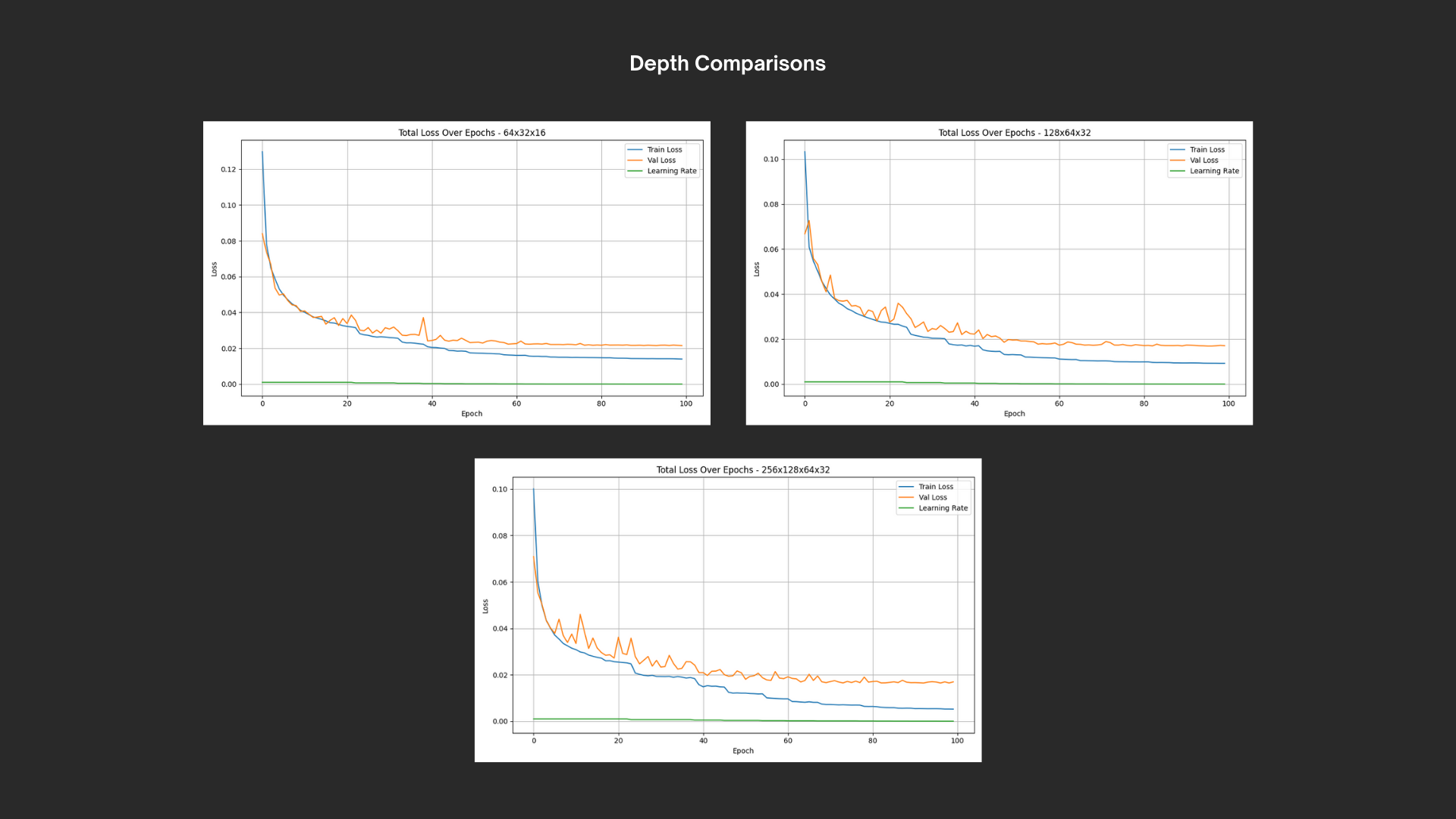
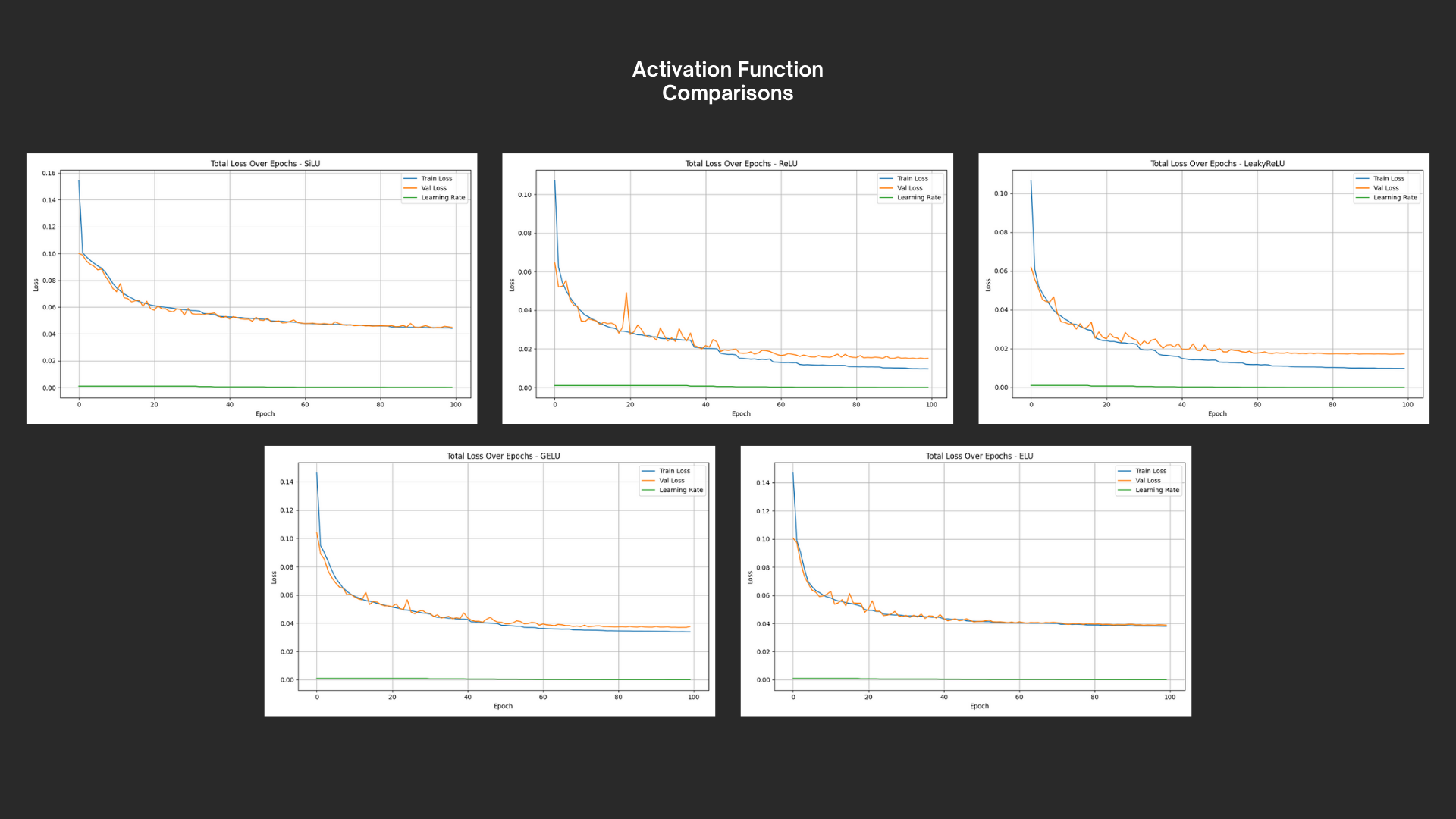
At this point, I was able to begin training without problem. For the first iteration of the architecture, I independently tested for optimal weight decay and learning rate scheduling, plotting and comparing results. After those were established, I tested varying model depth and lastly, using different activation functions. I wish I could say more about this, but in actuality it was just a matter of plotting and comparing results. With all of the discovered optimal parameters, I had a working MLP neural net that seemed generally successful at predicting collisions; In my validation set of length 21852, the model incorrectly predicted a collision that wasn’t due just 83 times and missed collisions that were supposed to occur a total of 23 times. This is an accuracy of about 99.51% - a figure I would consider initially successful. The collision classification head’s loss was also significantly higher than the other features, meaning that the model was even more successful at predicting the spatial data.
At this point, I felt as though I hadn’t pushed this project further than my pre-existing skillset. It was incredibly validating to see my current experience put into practice and so unproblematic at that - but my goal with this project was to explore and challenge myself. Thus far, I hadn’t really done so. Because of this, I decided to try and push to cross the gap between my current results and 100% accuracy.
In order to do so, I had to first diagnose what the model was having difficulty with rather than just throw hopeful ‘improvements’ at it. I began by adding an export to my testing flow that saved all the incorrect predictions to a csv file. In Houdini, I then added a node after the initial condition randomizations that overrides these attributes with the data in the error file. By manually incrementing a variable, the Houdini script would select a line of the csv, displaying the exact conditions that the model was unable to properly predict an outcome for. The hope was that visualizing the conditions of these predictions would reveal some problematic circumstance that I could account for somehow.
In doing this, I found a few different types of scenarios:
The balls are set to just barely miss each other, and the model incorrectly predicts there is a collision incoming. This is the most expected issue. Unfortunately, I imagine this will be the most difficult to solve as well since it’ll be a matter of increasing resolution on the learned boundary between collision conditions and otherwise.
Similarly, another scenario is: the balls visually seem to just barely hit but don’t penetrate enough that a collision is registered. The model predicts there’s a collision, which initially seems right. At first glance, I thought this was an issue in how the solver calculates collisions. In the bullet solver, there’s a scalable threshold of penetration before two objects are considered impacted, effectively making the radii of the spheres slightly smaller. However, the model’s ‘sight’ of these radii is only implicit anyways; it would always be learning the physical boundaries that are used for collision detection in generating the dataset. This means that this type of error scenario is in reality the same as the previous, even if it visually looks as though a collision occurs. This is significant because it means that in these cases, the model is technically outperforming my human eyes.
One ball is very closely and slowly trailing the other, and the model incorrectly predicts either way. This one is problematic because in simulating these conditions, I noticed that sometimes the end results didn’t match the dataset. I suspect this is because at slow rolling conditions, the spheres wobble based on their subdivision geometry. I’m not sure if I can get rid of this behavior entirely, but tightening parameters, increasing sub-steps, as well as geometry subdivisions should all raise classification accuracy. This should also help with the previous issue. Additionally, I will be implementing a check to ensure only up to one collision is allowed. Frankly, I had considered the possibility that the spheres will collide multiple times per simulation, but I expected this to be such an edge case that I would practically never see it nor have to worry about it. However, this wobbling behavior increases the likelihood a significant amount and I don’t want messy simulations to pollute my dataset.
The vector velocities of the two spheres point in similar direction despite the trajectories obviously not resulting in a collision. The model incorrectly predicts there’s an imminent collision. This seemed to be the most severe of the errors because unlike with the other two, I can visually discern the proper classification here. This puzzled me, because aside from these cases, the model appeared to be quite a lot better than me at predicting outcomes. However, this weakness makes perfect sense if you consider how I generated the dataset. Previously, when I had noticed the low collision frequency in my initial data, I added a brute-force override forcing the velocity directions to intersect as a means of artificially creating collisions. This worked in increasing the frequency, but it still didn’t make a collision occur every single time. In order to properly saturate my dataset, I had to also filter out the conditions where a collision didn’t occur, even with the brute-forcing. As a result, though, I inadvertently taught the model to correlate directional intersection with a collision without considering the velocity magnitude impact on trajectory nearly enough. This makes sense as I was removing the intersection conditions where collisions don’t occur — scenarios that would have been able to highlight the nuance. To solve this, I would have to generate another dataset with a different distribution, paying extra attention to including datapoints that not only entail collisions but near-collision misses. This would also improve accuracy with the other error cases as well, since I’d effectively be increasing the resolution on the learned boundary.

With the mentioned adjustments in mind, I am now working on generating a new revised dataset with the following simulation distributions:
Fully Natural Random Data - 15% (Regardless of collision outcome)
Semi-Catered Data - 85% (Linear interpolation between random and intersecting velocities)
0-1 interpolation - 20% (Regardless of collision outcome)
0.75-1 interpolation - 25% (Regardless of collision outcome)
0.9-1 interpolation - 25% (Regardless of collision outcome)
0.95-1 interpolation - 10% (Filtering out non-collision simulations)
0.975-1 interpolation - 5% (Filtering out non-collisions simulations and post-collision frames)
Even though 15% of the dataset is comprised of the 0.95-1 interpolation samples with non-collision simulation filtering, the post-collision frames will still point to no future impact. The samples with the post-collision frames removed will also just net much fewer frames in general. Because of this, I’m not sure what the frequency of collisions will be in terms of the frames themselves. As a result, if after generating these distributions, I have a collision frame frequency of less than 15%, I’ll keep simulating the 0.95-1 interpolation sample with both non-collisions simulation and post-collision frame filtering. I will also begin simulating with the assumption that 100% will correspond to 2000 simulations.
With the start of the academic year semester, this project is temporarily on pause until my schoolwork for the semester is over. There may be school projects taken on in the meantime, but this is my first priority once my final exams are taken.